NDT Matching with Autoware
Normal Distribution Transform (NDT)
3D maps enable self driving cars to localize themselves in the environment. To localize using a map and Lidar data one needs to find a way to associate the point cloud from the sensor with the point cloud from the map. This is also known as scan matching in robotics. One of the common ways to do this is Iterative Closest Point, it uses 6 degrees of freedom to find the closest point to the geometric entity from a given 3D point cloud. There exist a lot of geometric variants of ICP such as point-to-plane etc. One of the downfalls of ICP is that it needs a good approximation and a good starting point as it works on non-linear optimization and has tendencies to get stuck in local minima. In real world scenarios our points will probably be a little off from the map. Measurement errors will cause points to be slightly mis-aligned, plus the world might change a little between when we record the map and when we make our new scan. NDT matching provides a solution for these minor errors. Instead of trying to match points from our current scan to point on the map, we try to match points from our current scan to a grid of probability functions created from the map.
Following are the two tasks performed
-
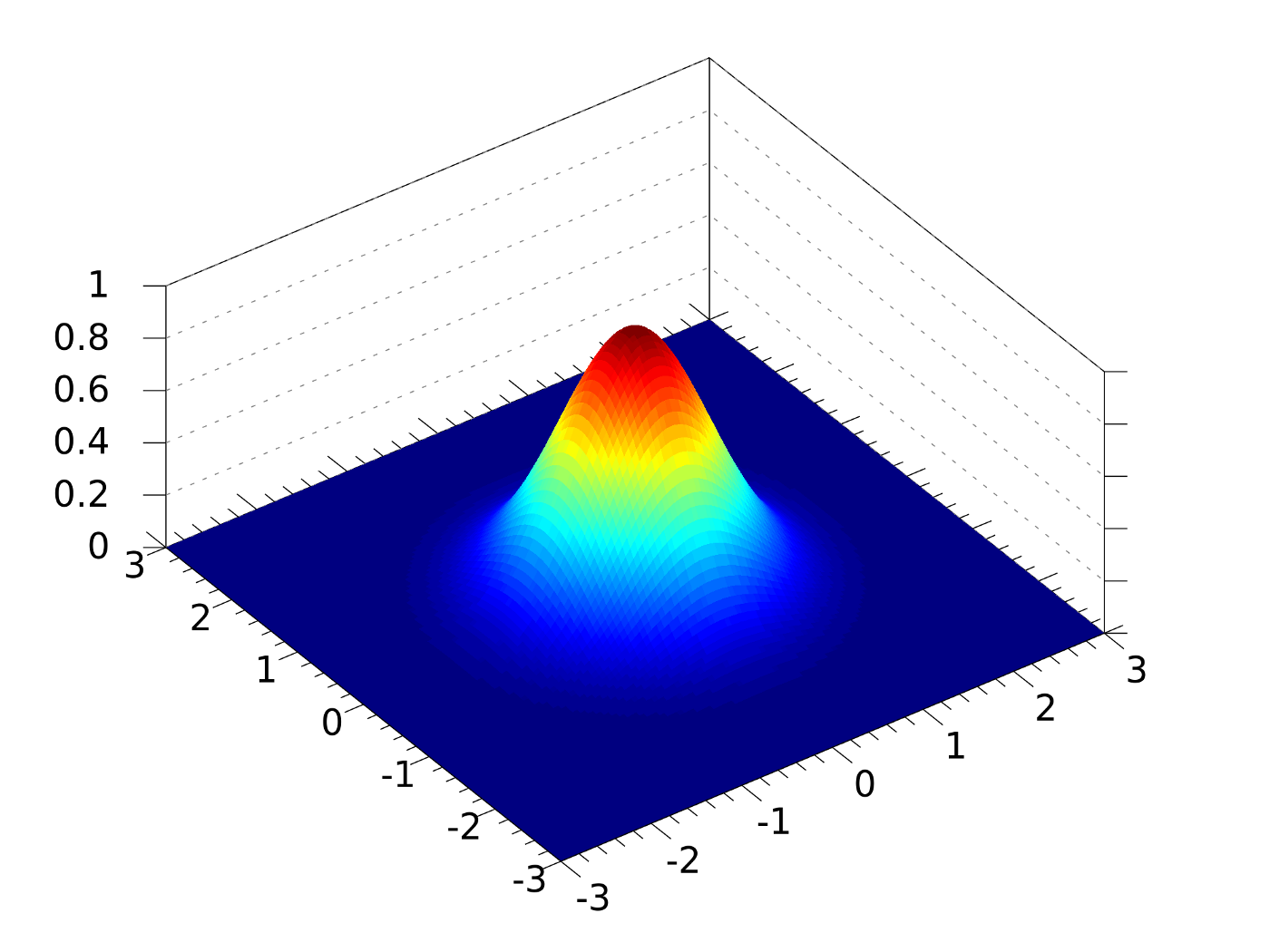
NDT mapping (Map generation) - Transform the LiDAR point cloud into a piecewise continuous and differentiable probability density (NDT). The probability density contains a set of the normal distributions where each point in point cloud is assigned to a voxel. A voxel is a 3D lattice cube to which points are assigned depending upon their coordinate value. The Point cloud is divided into k ND voxels clouds and are combined together , and also the voxel grid filter is used to decrease the computation cost and to reduce the noise from the 3D map
-
NDT matching (Localization) - A search problem where we have to find a transform that maximizes NDT sum to match the different point clouds, a variety of minimization functions can be used for this. Newton nonlinear optimizer is used to find the best 6-DOF pose.
Hardware Requirements
Velodyne VLP-16 and Computer running Autoware, some mobile platform with transforms known
Software
First, setup the Velodyne sensor(s) appropriately. If you are using multiple sensors, you will need to publish their relative transforms by using tf_static_publisher after obtaining these TFs using Autoware. see this blog post1. In case you just have one LIDAR, connect it to your laptop via wired Ethernet, and power it using a 8-20V DC power input (battery pack works), a VLP-16 consumes about 8W. Then you need to set up your laptop with a static IP configuration, meaning that the wired connection should be on the 192.168.1.* subnet, and your LIDAR default IP address will be 192.168.1.201. You can reconfigure this if you are using multiple LIDARs, as described in the above blog post. You need to initialize the LIDAR in the ROS framework by using the following ROS command (VLP-16), make sure you have the ros_velodyne_driver package installed for this to work successfully.
roslaunch velodyne_pointcloud VLP16_points.launch
You can check that the above node is publishing by doing a “rostopic echo” for the /velodyne_points topic. Troubleshooting if it isn’t working - check the IP address, see if the Ethernet is configured correctly on your laptop, see if you are able to ping the sensor (ping 192.168.1.201 or the IP address that you have set), see if it is powered on and spinning (hold your hand on top of the sensor and you should feel the motor spinning). Once the Velodyne LIDAR is publishing data, you can go ahead with the ROSbag collection as described below. If you want to incorporate additional sensor information like the IMU or GPS, just install the relevant ROS drivers for the sensors and ensure that they publish data onto the standard /imu_raw or /nmea (incomplete topic name) topics as required by Autoware. Launch Autoware using the runtime_manager as follows:
source autoware/install/setup.bash
roslaunch runtime_manager runtime_manager.launch
You need to create a ROSBag of the space that you would like to map, so click on the ROSbag button on the bottom right of the main Autoware Runtime Manager console. Choose the topics that are relevant for your mapping (like /velodyne_points, /imu_raw, /nmea, etc.) and then start recording while moving the vehicle/robot very slowly through the space. If the space is really large (campus-sized or larger) then you might want to split the ROSbags to ensure that it does not fail to complete mapping at a later stage (large ROS messages cause ndt mapping to fail, and large ROSbags may be problematic to load/store/replay). Once you have created the ROSbag, you can visualize the output of your “random walk” by replaying the ROSbag and opening Rviz to view the pointcloud that was generated at each position: rosbag play the_rosbag_you_just_saved.bag
rosrun rviz rviz -f velodyne # assuming you had a velodyne frame
Video reference for rest of this post To start creating the map, launch the NDT Mapping node in Autoware by clicking on it in the Computing tab (also specify any additional sensors you used like GPS or IMU, and for the rest, default parameters are fine). Then run the ROSbag but remap your velodyne_points to /points_raw since that is what Autoware uses for the ndt_mapping node. So something like below:
rosbag play the_rosbag_you_just_saved.bag /velodyne_points:=/points_raw
Then you will see the mapping running really quickly in one terminal and the number of point-cloud poses being considered (there will be 10 every second because that is the frequency of rotation of the LIDAR). Once the full ROSbag has played, wait for all the poses to be fused into the map, because sometimes when the map is really large, the mapping might not have caught up with the ROSbag running. Additionally, when you have a very large map, use approximate_ndt_mapping instead, refer to blog post 2 here.
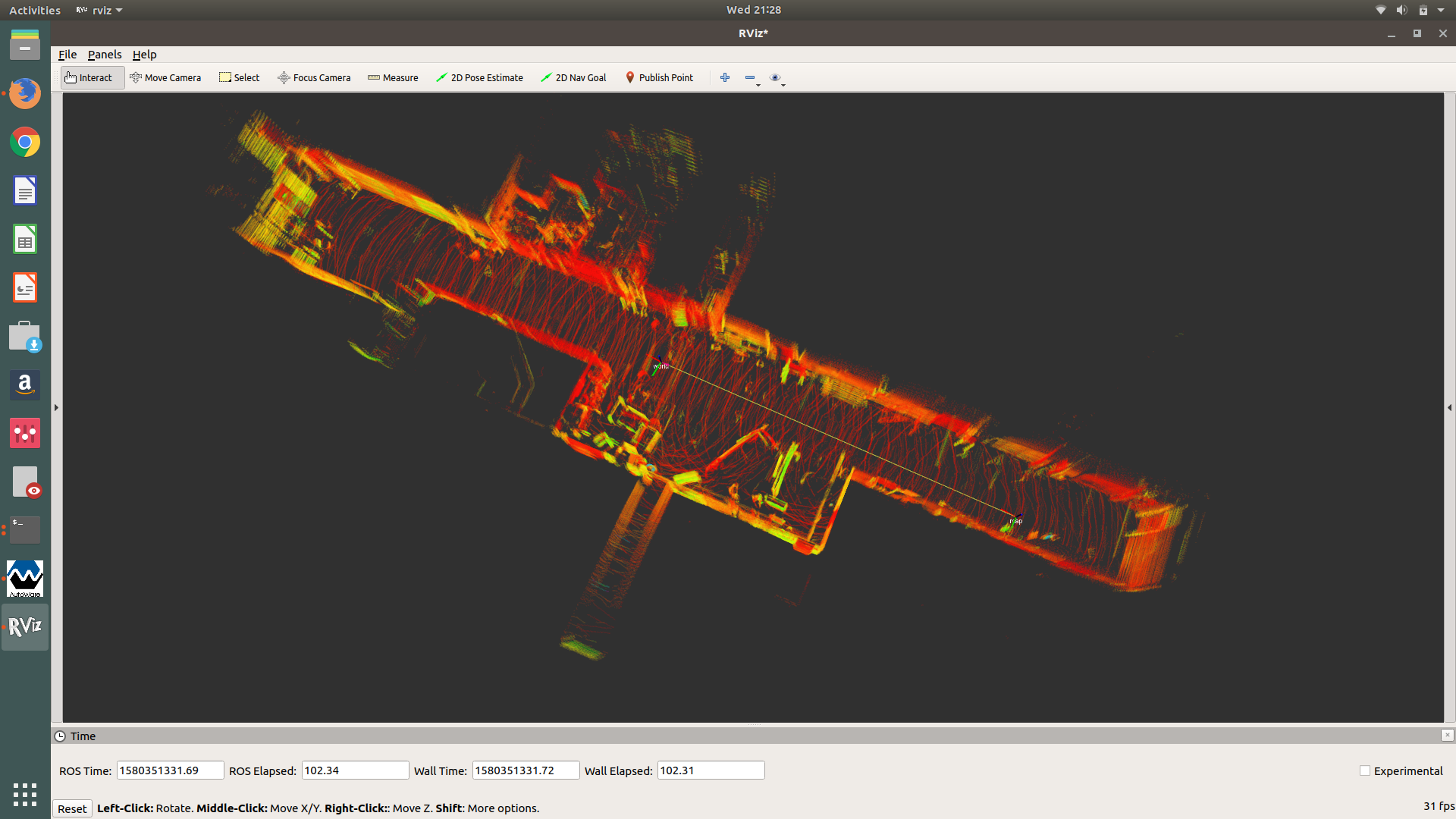
Once you have finished creating the map, save it in your desired location with either a downsampling (to reduce the file size), or full/original quality output, by using the “app” tab in the NDT_Mapping node in the Computing tab. It will save as a .pcd file that can either be viewed using PCL_Viewer (a PCL tool) or RViz with Autoware. The image below shows a map we made of NSH B-level on 29th January, 2020. To view a map in RViz, load Autoware, initialize the point cloud in the Mapping tab, and click on the TF button for a default TF. Then you should be able to launch RViz and visualize the point_map as shown below. You can change the point colours and axis colours to “intensity” and the sizes/transparencies as well.