Guassian Process and Gaussian Mixture Model

This document acts as a tutorial on Gaussian Process(GP), Gaussian Mixture Model, Expectation Maximization Algorithm. We recently ran into these approaches in our robotics project that having multiple robots to generate environment models with minimum number of samples.

You will be able to have a basic understanding on Gaussian Process (what is it and why it is very popular), Gaussian Mixture Model and Expectation Maximization Algorithm after this tutorial.

Gausssian Process
Gaussian Mixture Model
Expectation Maximization Algorithm
Summary
References

Gausssian Process

What is GP?

A Gaussian Process(GP) is a probability distribution over functions \( p(\textbf{f}) \) , where the functions are defined by a set of random function variables \(\textbf{f} = {f_1, f_2, . . . , f_N}\). For a GP, any finite linear combination of those function variables has a joint (zero mean) Gaussian distribution. It can be used for nonlinear regression, classification, ranking, preference learning, ordinal regression. In robotics, it can be applied to state estimation, motion planning and in our case environment modeling.

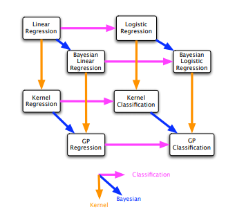
GPs are closely related to other models and can be derived using bayesian kernel machines, linear regression with basis functions, infinite multi-layer perceptron neural networks (it becomes a GP if there are infinitely many hidden units and Gaussian priors on the weights), spline models. A simple connections between different methods can be found in the following figure.

Before all the equations, lets have a look at why do we want to use GP?

Why do we want to use GP?

The major reasons why GP is popular includes:

It can handle uncertainty in unknown function by averaging, not minimizing as GP is rooted in probability and bayesian inference. 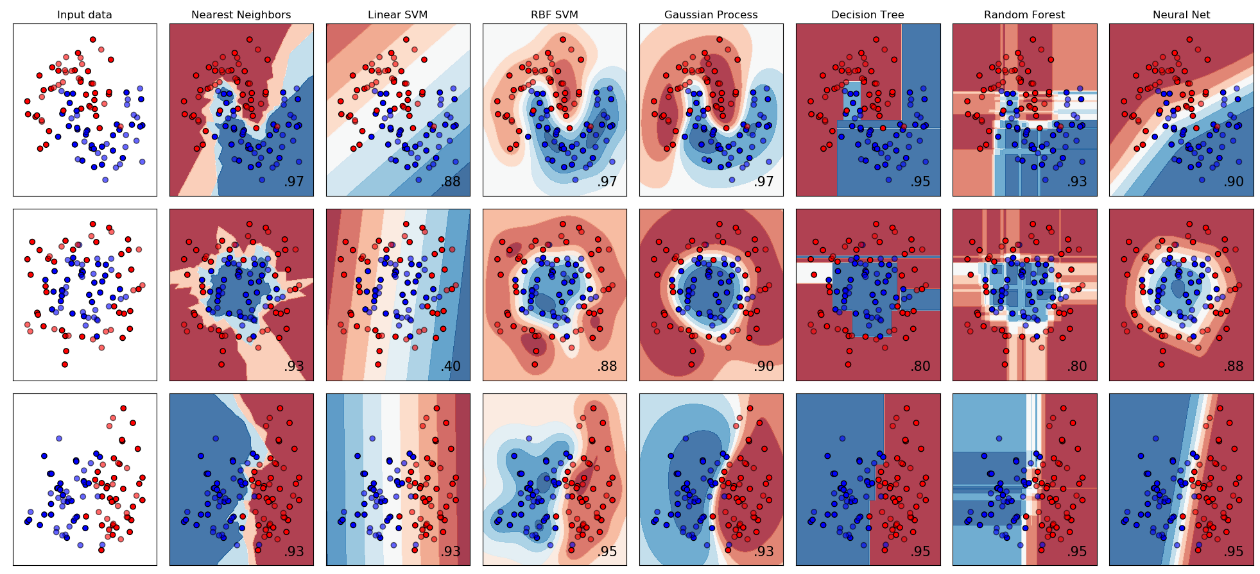Classifier comparison(https://scikit-learn.org/stable/auto_examples/classification/plot_classifier_comparison.html) This property is not commonly shared by other methods. For example, in the above classification method comparison. Neural nets and random forests are confident about the points that are far from the training data.
We can incorporate prior knowledge by choosing different kernels
GP can learn the kernel and regularization parameters automatically during the learning process. (GP is a non-parametric model, but all data are needed to generate the model. In other words, it need finite but unbounded number of parameters that grows with data.)
It can interpolate training data.

Gaussian Process for Regression

In this section, we will show how to utilize GP for solving regression problems. The key idea is to map the independent variables from low-dimensional space to high-dimensional space. The idea is similar to the kernel function in support vector machine, where the linear-inseparable data in the low-dimensional space can be mapped to a high-dimensional where the data can be separated by a hyper-plane.

When using Gaussian process regression, there is no need to specify the specific form of f(x), such as \( f(x)=ax^2+bx+c \). The observations of n training labels \( y_1, y_2, …, y_n \) are treated as points sampled from a multidimensional (n-dimensional) Gaussian distribution.

For a given training examples \( x_1, x_2, …, x_n \) and the corresponding observations \(y_1, y_2, …, y_n \), the target \( y \) can be modeled by an implicit function \(f(x)\). Since the observations are usually noisy, each observation y is added with a Gaussian noise.

\[ y = f(x) + N(0, \sigma^2_n) \]

\( f(x) \) is assumed to have a prior \( f(x) \sim GP(0,K_{xx}) \), where \(K_{xx}\) is the covariance matrix. There are multiple method to formulate the covariance here. You can also use a combination of covariance functions. Since the mean is assumed to be zero, the final result depends largely on the choice of covariance function.

Suppose we have a dataset containing \( n \) training examples \( (x_i, y_i) \), and we want to predict the value \( y^* \) given \( x^* \). After adding the unknown value, we get a variable of \( (n+1) \) dimension.

\[\left[\begin{array}{c} y_{1} \\ \vdots \\ y_{n} \\ f\left(x^{*}\right) \end{array}\right] \sim \mathcal{N}\left(\left[\begin{array}{c} 0 \\ 0 \end{array}\right],\left[\begin{array}{cc} K_{x x}+\sigma_{n}^{2} I & K_{x x}^{T} \\ K_{x x}^{2} & k\left(x^{*}, x^{*}\right) \end{array}\right]\right)\]

where,

\[K_{x x^{* }}=\left[k\left(x_{1}, x^{* }\right) \ldots k\left(x_{n}, x^{* }\right)\right ] \]

Hence, the problem can be convert into a conditional probability problem, i.e. solving \( f(x^* )|\mathbf{y}(\mathbf{x}) \).

\[ f\left(x^{* }\right) | \mathbf{y}(\mathbf{x}) \sim \mathcal{N}\left(K_{x x^{* }} M^{-1} \mathbf{y}(\mathbf{x}), k\left(x^{* }, x^{* }\right)-K_{x x^{* }} M^{-1} K_{x^{* } x}^{T}\right)\]

where \( M=K_{x x}+\sigma_{n}^{2} I \), hence the expectation of \( y^* \) is

\[ E\left(y^{* }\right)=K_{x x^{* }} M^{-1} \mathbf{y}(\mathbf{x})\]

The variance is \[ \operatorname{Var}\left(y^{* }\right)=k\left(x^{* }, x^{* }\right)-K_{x x^{* }} M^{-1} K_{x^{* } x}^{T}\]

Gaussian Mixture Model

Mixture model

The mixture model is a probabilistic model that can be used to represent K sub-distributions in the overall distribution. In other words, the mixture model represents the probability distribution of the observed data in the population, which is a mixed distribution consisting of K sub-distributions. When calculating the probability of the observed data in the overall distribution, the mixture model does not require the information about the sub-distribution in the observation data.

Gaussian Model

When the sample data X is univariate, the Gaussian distribution follows the probability density function below. \[ P(x|\theta)=\frac{1}{\sqrt{2\pi \sigma^2}}exp(-\frac{(x-\mu)^2}{2\sigma^2}) \]

While \( \mu \) is the average value of the data (Expectations), \( \sigma \) is the standard deriviation.

When the sample data is multivariate, the Gaussian distribution follows the probability density function below. \[ P(x|\theta)=\frac{1}{(2\pi)^{\frac{D}{2}} |\Sigma|^{\frac{1}{2}}}exp(-\frac{(x-\mu)^T\Sigma^{-1}(x-\mu)}{2}) \]

While \( \mu \) is the average value of the data (Expectations), \( \Sigma \) is the covariance, D is the dimention of the data.

Gaussian Mixture Model

The Gaussian mixture model can be regarded as a model composed of K single Gaussian models, which are hidden variables of the hybrid model. In general, a mixed model can use any probability distribution. The Gaussian mixture model is used here because the Gaussian distribution has good mathematical properties and good computational performance.

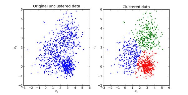
For example, we now have a bunch of samples of dogs. Different types of dogs have different body types, colors, and looks, but they all belong to the dog category. At this time, the single Gaussian model may not describe the distribution very well since the sample data distribution is not a single ellipse. However, a mixed Gaussian distribution can better describe the problem, as shown in the following figure:

Define:

\( x_j \) is the number \( j \) of the observed data, \( j = 1, 2, …, N \)
\( k \) is the number of Gaussians in the mixture model, \( k = 1, 2, …, K \)
\( \alpha_k \)is the probability that the observed data is from the \( k \)th gaussian, \( \alpha_k > 0 \), \( \Sigma_{k=1}^{K}\alpha_k=1 \)
\( \phi(x|\theta_k) \) is the gaussian density function of the \( k \)th sub-model, \( \theta_k = (\mu, \sigma^2_k) \)
\( \gamma_{jk} \) is the probability that the \( j \)th observed data is from the \( k \)th gaussian.

The probablity distribution of the gaussian mixture model: \[ P(x|\theta)= \Sigma^K_{k=1} \alpha_k\phi(x|\theta_k) \]

As for this model, \( \theta = (\mu_k, \sigma_k, \alpha_k) \), which is the expectation, standard deriviation (or covariance) and the probability of the mixture model.

Learning the parameters of the model

As for the single, we can use Maximum Likelihood to estimate the value of parameter \( \theta \) \[ \theta = argmax_\theta L(\theta) \]

We assume that each data point is independent and the likelihood function is given by the probability density function. \[ L(\theta) = \Pi^N_{j=1}P(x_j|\theta) \]

Since the probability of occurrence of each point is very small, the product becomes extremely small, which is not conducive to calculation and observation. Therefore, we usually use Maximum Log-Likelihood to calculate (because the Log function is monotonous and does not change the position of the extreme value, At the same time, a small change of the input value can cause a relatively large change in the output value): \[ logL(\theta) = \Sigma^N_{j=1}logP(x_j|\theta) \]

As for the Gaussian Mixture Model, the Log-likelihood function is: \[ logL(\theta) = \Sigma^N_{j=1}logP(x_j|\theta) = \Sigma^N_{j=1}log(\Sigma^K_{k=1})\alpha_k \phi(x|\theta_k) \]

So how do you calculate the parameters of the Gaussian mixture model? We can’t use the maximum likelihood method to find the parameter that maximizes the likelihood like the single Gaussian model, because we don’t know which sub-distribution it belongs to in advance for each observed data point. There is also a summation in the log. The sum of the K Gaussian models is not a Gaussian model. For each submodel, there is an unknown \( (\mu_k, \sigma_k, \alpha_k) \), and the direct derivation cannot be calculated. It need to be solved by iterative method.

Expectation Maximization Algorithm

The EM algorithm is an iterative algorithm, summarized by Dempster et al. in 1977. It is used as a maximum likelihood estimation of probabilistic model parameters with Hidden variables.

Each iteration consists of two steps:

E-step: Finding the expected value \( E(\gamma_{jk}|X,\theta) \) for all \( j = 1, 2, …, N \)
M-step: Finding the maximum value and calculate the model parameters of the new iteration

The general EM algorithm is not specifically introduced here (the lower bound of the likelihood function is obtained by Jensen’s inequality, and the maximum likelihood is maximized by the lower bound). We will only derive how to apply the model parameters in the Gaussian mixture model.

The method of updating Gaussian mixture model parameters by EM iteration (we have sample data \( x_1, x_2, …, x_N \) and a Gaussian mixture model with \( K\) submodels, we want to calculate the optimal parameters of this Gaussian mixture model):

Initialize the parameters
E-step: Calculate the possibility that each data \( j\) comes from the submodel \( k\) based on the current parameters \[ \gamma_{jk} = \frac{\alpha_k\phi(x_j|\theta_k)}{\Sigma_{k=1}^K\alpha_k\phi(x_j|\theta_k)}, j=1 , 2,…,N; k=1, 2, …, K \]
M-step: Calculate model parameters for a new iteration \[ \mu_k = \frac{\Sigma_j^N(\gamma_{jk}x_j)}{\Sigma_j^N\gamma_{jk}}, k=1,2,…,K \] \[ \Sigma_k = \frac{\Sigma_j^N\gamma_{jk}(x_j-\mu_k)(x_j-\mu_k)^T}{\Sigma_j^N\gamma_{jk}}, k=1,2,…,K \] \[ \alpha_k = \frac{\Sigma_j^N\gamma_{jk}}{N}, k=1,2,…,K \]
Repeat the calculation of E-step and M-step until convergence (\( ||\theta_{i+1}-\theta_i||<\epsilon \), \( \epsilon \) is a small positive number, indicating that the parameter changes very small after one iteration)

At this point, we have found the parameters of the Gaussian mixture model. It should be noted that the EM algorithm has a convergence, but does not guarantee that the global maximum is found since it is possible to find the local maximum. The solution is to initialize several different parameters to iterate and take the best result.

Summary

A Gaussian Process(GP) is a probability distribution over functions. It can be used for nonlinear regression, classification, ranking, preference learning, ordinal regression. In robotics, it can be applied to state estimation, motion planning and in our case environment modeling. It has the advantages of learning the kernel and regularization parameters, uncertainty handling, fully probabilistic predictions, interpretability.

The Gaussian mixture model (GMM) can be regarded as a model composed of K single Gaussian models, which are hidden variables of the hybrid model. It utilizes Gaussian’s good mathematical properties and good computational performance.

Expectation Maximization Algorithm (EM) is a iterative algorithm that act as a maximum likelihood estimation of probabilistic model parameters with Hidden variables.

References

C. E. Rasmussen and C. K. I. Williams. Gaussian Processes for Machine Learning. MIT Press,2006.
An intuitive guide to Gaussian processes: http://asctecbasics.blogspot.com/2013/06/basic-wifi-communication-setup-part-1.html
Qi, Y., Minka, T.P., Picard, R.W., and Ghahramani, Z. Predictive Automatic Relevance Determination by Expectation Propagation. In Twenty-first International Conference on Machine Learning (ICML-04). Banff, Alberta, Canada, 2004.
O’Hagan, A. Curve Fitting and Optimal Design for Prediction (with discussion). Journal of the Royal Statistical Society B, 40(1):1-42, 1978.
MacKay, David, J.C. (2003). Information Theory, Inference, and Learning Algorithms. Cambridge University Press. p. 540. ISBN 9780521642989.
Dudley, R. M. (1975). “The Gaussian process and how to approach it”. Proceedings of the International Congress of Mathematicians.
Bishop, C.M. (2006). Pattern Recognition and Machine Learning. Springer. ISBN 978-0-387-31073-2.
Dempster, A.P.; Laird, N.M.; Rubin, D.B. (1977). “Maximum Likelihood from Incomplete Data via the EM Algorithm”. Journal of the Royal Statistical Society, Series B. 39 (1): 1–38. JSTOR 2984875. MR 0501537.
“Maximum likelihood theory for incomplete data from an exponential family”. Scandinavian Journal of Statistics. 1 (2): 49–58. JSTOR 4615553. MR 0381110.

Guassian Process and Gaussian Mixture Model

Table of Contents

Gausssian Process

What is GP?

Why do we want to use GP?

Gaussian Process for Regression

Gaussian Mixture Model

Mixture model

Gaussian Model

Gaussian Mixture Model

Learning the parameters of the model

Expectation Maximization Algorithm

Summary

Further Reading

References