YOLOv5 Training and Deployment on NVIDIA Jetson Platforms
Object detection with deep neural networks has been a crucial part of robot perception. Among object detection models, single-stage detectors, like YOLO, are typically more lightweight and suitable for mobile computing platforms. In the meantime, NVIDIA has developed the Jetson computing platforms for edge AI applications, supporting CUDA GPU acceleration. Compared with desktop or laptop GPUs, Jetson’s GPUs have lower computation capacity; therefore, more care should be taken on the selection of neural network models and fine-tuning on both speed and performance.
This article uses YOLOv5 as the objector detector and a Jetson Xavier AGX as the computing platform. It will cover setting up the environment, training YOLOv5, and the deployment commands and code. Please note that unlike the deployment pipelines of previous YOLO versions, this tutorial’s deployment of YOLOv5 doesn’t rely on darknet_ros, and at runtime, the program only relies on C++, ROS, and TensorRT.
Jetson Xavier AGX Setup
Setting up the Jetson Xavier AGX requires an Ubuntu host PC, on which you need to install the NVIDIA SDK Manager. This program allows you to install Jetpack on your Jetson, which is a bundled SDK based on Ubuntu 18.04 and contains important components like CUDA, cuDNN and TensorRT. Note that as of 2021, Jetpack does not officially support Ubuntu 20.04 on the Jetsons. Once you have the SDK Manager ready on your Ubuntu host PC, connect the Jetson to the PC with the included USB cable, and follow the onscreen instructions.
Note that some Jetson models including the Xavier NX and Nano require the use of an SD card image to set up, as opposed to a host PC.
After setting up your Jetson, you can then install ROS. Since Jetson runs on Ubuntu 18.04, you’ll have to install ROS Melodic. Simply follow the instructions on rog.org: ROS Melodic Installation
Training YOLOv5 or Other Object Detectors
A deep neural net is only as good as the data it’s been trained on. While there are pretrained YOLO models available for common classes like humans, if you need your model to detect specific objects you will have to collect your own training data.
For good detection performance, you will need at least 1000 training images or more. You can collect the images with any camera you would use, including your phone. However, you need to put a lot of thought into where and how you’ll take the images. What type of environment will your robot operate in? Is there a common backdrop that the robot will see the class objects in? Is there any variety among objects of the same class? What distance/angle will the robot see the objects from? The answers to these questions will heavily inform your ideal dataset. If your robot will operate in a variety of indoor/outdoor environments with different lighting conditions, your dataset should have similar varieties (and in general, more variety = more data needed!). If your robot will only ever operate in a single room and recognize only two objects, then it’s not a bad idea to take images of only these two objects only in that room. Your model will overfit to that room in that specific condition, but it will be a good model if you’re 100% sure it’s the only use case you ever need. If you want to reinforce your robot’s ability to recognize objects that are partially occluded, you should include images where only a portion of the object is visible. Finally, make sure your images are square (1:1 aspect ratio, should be an option in your camera app). Neural nets like square images, and you won’t have to crop, pad or resize them which could undermine the quality of your data.
Once you have your raw data ready, it’s time to process them. This includes labeling the classes and bounding box locations as well as augmenting the images so that the model trained on these images are more robust. There are many tools for image processing, one of which is Roboflow which allows you to label and augment images for free (with limitations, obviously). The labeling process will be long and tedious, so put on some music or podcasts or have your friends or teammates join you and buy them lunch later. For augmentation, common tricks include randomized small rotations, crops, brightness/saturation adjustments, and cutouts. Be sure to resize the images to a canonical size like 416x416 (commonly used for YOLO). If you feel that your Jetson can handle a larger image size, try something like 640x640, or other numbers that are divisible by 32. Another potentially useful trick is to generate the dataset with the same augmentations twice; you will get two versions of the same dataset, but due to the randomized augmentations the images will be different. Like many deep learning applications, finding the right augmentations involves some trial-and-error, so don’t be afraid to experiment!
Once you have the dataset ready, time to train! Roboflow has provided tutorials in the form of Jupyter Notebooks, which contains all the repos you need to clone, all the dependencies you need to install, and all the commands you need to run:
- The old version of the training jupyter notebook (The version that the authors tested on)
- The new version of the training jupyter notebook (A newer version published by Roboflow)
After training is finished, the training script will save the model weights to a .pt file, which you can then transform to a TensorRT engine.
Transforming a Pytorch Model to a TensorRT Engine
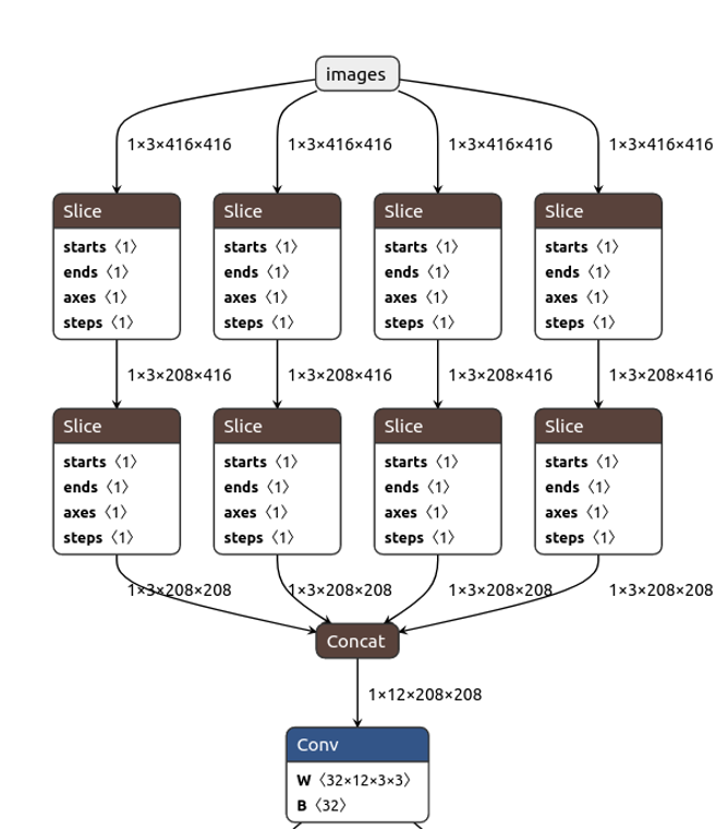
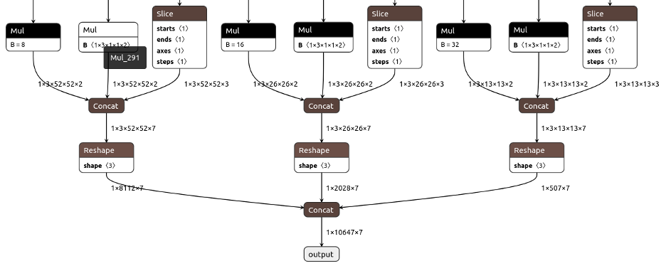
YOLOv5’s official repository provides an exporting script, and to simplify the post-processing steps, please checkout a newer commit, eg. “070af88108e5675358fd783aae9d91e927717322”. At the root folder of the repository, run python export.py --weights WEIGHT_PATH/WEIGHT_FILE_NAME.pt --img IMAGE_LENGTH --batch-size 1 --device cpu --include onnx --simplify --opset 11. There’ll be a .onnx file generated next to the .pt file, and netron provides a tool to easily visualize and verify the onnx file. For example, if the image size is 416x416, the model is YOLOv5s and the class number is 2, you should see the following input and output structures:
After moving the .onnx file to your Jetson, run trtexec --onnx=ONNX_FILE.onnx --workspace=4096 --saveEngine=ENGINE_NAME.engine --verbose to obtain the final TensorRT engine file. The 4096 is the upper bound of the memory usage and should be adapted according to the platform. Besides, if there’s no trtexec command while TensorRT was installed, add export PATH=$PATH:/usr/src/tensorrt/bin to your ~/.bashrc or ~/.zshrc, depending on your default shell.
You don’t need to specify the size of the model here, because the input and output sizes have been embedded into the onnx file. For advanced usage, you may specify the dynamic axes on your onnx file, and at the trtexec step, you should add --explicitBatch --minShapes=input:BATCH_SIZExCHANNELxHEIGHTxWIDTH --optShapes=input:BATCH_SIZExCHANNELxHEIGHTxWIDTH --maxShapes=input:BATCH_SIZExCHANNELxHEIGHTxWIDTH .
To achieve better inference speed, you can also add the --fp16 flag. This could theoretically reduce 50% of the computation time.
Integrating TensorRT Engines into ROS
First, under a ROS package, add the following content to your CMakeLists.txt
find_package(CUDA REQUIRED)
message("-- CUDA version: ${CUDA_VERSION}")

find_package(OpenCV REQUIRED)

# cuda
include_directories(/usr/local/cuda/include)
link_directories(/usr/local/cuda/lib64)
# tensorrt
include_directories(/usr/include/aarch64-linux-gnu/)
link_directories(/usr/lib/aarch64-linux-gnu/)
For the executable or library running the TensorRT engine, in target_include_directories, add \${OpenCV_INCLUDE_DIRS} \${CUDA_INCLUDE_DIRS}, and in target_link_libraries, add \${OpenCV_LIBS} nvinfer cudart.
In the target c++ file, create the following global variables. The first five variables are from TensorRT or CUDA, and the other variables are for data input and output. The sample::Logger is defined in logging.h, and you can download that file from TensorRT’s Github repository in the correct branch. For example, this is the link to that file for TensorRT v8.
sample::Logger gLogger;
nvinfer1::ICudaEngine *engine;
nvinfer1::IExecutionContext *context;
nvinfer1::IRuntime *runtime;
cudaStream_t stream;
Beyond that, you should define the GPU buffers and CPU variables to handle the input to and output from the GPU. The buffer size is 5 here because there are one input layer and four output layers in the onnx file. INPUT_SIZE and OUTPUT_SIZE are equal to their batch_size * channel_num * image_width * image_height.
constexpr int BUFFER_SIZE = 5;
// buffers for input and output data
std::vector<void *> buffers(BUFFER_SIZE);
std::shared_ptr<float[]> input_data
  = std::shared_ptr<float[]>(new float[INPUT_SIZE]);
std::shared_ptr<float[]> output_data
  = std::shared_ptr<float[]>(new float[OUTPUT_SIZE]);
Before actually running the engine, you need to initialize the “engine” variable, and here’s an example function. This function will print the dimensions of all input and output layers if the engine is successfully loaded.
void prepareEngine() {
  const std::string engine_path = “YOUR_ENGINE_PATH/YOUR_ENGINE_FILE_NAME";
  ROS_INFO("engine_path = %s", engine_path.c_str());
  std::ifstream engine_file(engine_path, std::ios::binary);

  if (!engine_file.good()) {
	ROS_ERROR("no such engine file: %s", engine_path.c_str());
	return;
  }

  char *trt_model_stream = nullptr;
  size_t trt_stream_size = 0;
  engine_file.seekg(0, engine_file.end);
  trt_stream_size = engine_file.tellg();
  engine_file.seekg(0, engine_file.beg);
  trt_model_stream = new char[trt_stream_size];
  assert(trt_model_stream);
  engine_file.read(trt_model_stream, trt_stream_size);
  engine_file.close();

  runtime = nvinfer1::createInferRuntime(gLogger);
  assert(runtime != nullptr);
  engine = runtime->deserializeCudaEngine(trt_model_stream, trt_stream_size);
  assert(engine != nullptr);
  context = engine->createExecutionContext();
  assert(context != nullptr);
  if (engine->getNbBindings() != BUFFER_SIZE) {
	ROS_ERROR("engine->getNbBindings() == %d, but should be %d",
          	engine->getNbBindings(), BUFFER_SIZE);
  }

  // get sizes of input and output and allocate memory required for input data
  // and for output data
  std::vector<nvinfer1::Dims> input_dims;
  std::vector<nvinfer1::Dims> output_dims;
  for (size_t i = 0; i < engine->getNbBindings(); ++i) {
	const size_t binding_size =
    	getSizeByDim(engine->getBindingDimensions(i)) * sizeof(float);
	if (binding_size == 0) {
  	ROS_ERROR("binding_size == 0");

  	delete[] trt_model_stream;
  	return;
	}

	cudaMalloc(&buffers[i], binding_size);
	if (engine->bindingIsInput(i)) {
  	input_dims.emplace_back(engine->getBindingDimensions(i));
  	ROS_INFO("Input layer, size = %lu", binding_size);
	} else {
  	output_dims.emplace_back(engine->getBindingDimensions(i));
  	ROS_INFO("Output layer, size = %lu", binding_size);
	}
  }

  CUDA_CHECK(cudaStreamCreate(&stream));

  delete[] trt_model_stream;

  ROS_INFO("Engine preparation finished");
}
At runtime, you should first copy the image data into the input_data variable. The following code snippet shows a straightforward solution. Please note that OpenCV’s cv::Mat has HWC (height - width - channel) layout, while TensorRT by default takes BCHW (Batch - channel - height - width) layout data.
  int i = 0;
  for (int row = 0; row < image_size; ++row) {
	for (int col = 0; col < image_size; ++col) {
  	input_data.get()[i] = image.at<cv::Vec3f>(row, col)[0];
  	input_data.get()[i + image_size * image_size] =
      	image.at<cv::Vec3f>(row, col)[1];
  	input_data.get()[i + 2 * image_size * image_size] =
      	image.at<cv::Vec3f>(row, col)[2];
  	++i;
	}
  }
Then, you can use the following lines of code to run the engine through its context object. The first line copies the input image data into buffers[0]. The second last line copies buffers[4], the combined bounding box output layer, to our output_data variable. In our onnx file example, this layer corresponds to 1 batch_size, 10647 bounding box entries, and 7 parameters describing each bounding box. The 7 parameters are respectively tx, ty, tw, th, object confidence value, and the two scores for the two classes, where tx, ty, tw and th means the center x, center y, width, and height of the bounding box.
  CUDA_CHECK(cudaMemcpyAsync(buffers[0], input_data.get(),
                         	input_size * sizeof(float), cudaMemcpyHostToDevice,
                         	stream));
  context->enqueue(1, buffers.data(), stream, nullptr);
  CUDA_CHECK(cudaMemcpyAsync(output_data.get(), buffers[4],
                         	output_size * sizeof(float),
                         	cudaMemcpyDeviceToHost, stream));
  cudaStreamSynchronize(stream);
The last step is the non-maximum suppression for those bounding boxes. Separately store bounding boxes according to their class id, and only keep boxes with object confidence values higher than a predefined threshold, eg. 0.5. Sort the bounding boxes from higher confidence value to lower ones, and for each bounding box, remove others with lower confidence values and intersection over union (IOU) higher than another predefined threshold, eg. 40%. To understand better about this process, please refer to non-maximum explanation.
The code of the above deployment process is available on Github.