Overview of Motion Planning

The problem of motion planning can be stated as follows: to find an optimal path for the robot to move through gradually from start to goal while avoiding any obstacles in between, given - a start pose of the robot a desired goal pose a geometric description of the robot a geometric description of the world

This Wiki details the different types of motion planning algorithms that are available and the key differences between them. Knowing this will make choosing between them easier, depending on the types of projects these algorithms are implemented in.

Search-Based Planning Algorithms:

This section is focused on search-based planning algorithms, and more specifically it is a very brief overview of two of the most popular search algorithms for robotic systems: A* and D* Lite. At the end of their respective sections, we have provided references to external resources where each algorithm and sufficient information to successfully implement each is provided. One critical thing to keep in mind is that A* searches from the start to the goal and D* Lite searches from the goal to the start. Memoization can save a significant amount of computation so consider which direction of search will allow keeping a longer portion of the path between search iterations for your application.

A*:

The A* algorithm is similar to Djikstra’s algorithm except that A* is incentivized to search towards the goal, thereby focusing the search. Specifically, the difference is an added heuristic that takes into account the cost of the node of interest to the goal node in addition to the cost to get to that node from the start node. Since A* prioritizes searching those nodes that are closer to the end goal, this typically results in faster computation time in comparison to Djikstra’s.

Graph search algorithms like Djikstra’s and A* utilize a priority queue to determine which node in the graph to expand from. Graph search models use a function to assign a value to each node, and this value is used to determine which node to next expand from. The function is of the form: f(s) = g(s) + h(s)

With g(s) being the cost of the path to the current node, and h(s) some heuristic which changes depending on which algorithm is being implemented. A typically used heuristic is euclidean distance from the current node to the goal node.

In Djikstra’s, the node with the lowest cost path from the start node is placed at the top of the queue. This is equivalent to not having any added heuristic h(s). In A*, the node with the lowest combined path cost to a node and path cost from the node to the goal node is placed at the top of the queue. In this case, the added heuristic h(s) is the path cost from the current node to the goal node. This heuristic penalizes nodes that are further from the goal even if during runtime of the algorithm these nodes have a relatively lower cost to reach from the start node. This is how A* is faster in computation time compared to Djikstra’s.

Depending on the heuristic used for calculating cost from a node to the end goal, computation time can vary. It is also important to use a heuristic that does not overestimate the cost to the end goal, otherwise the algorithm may never expand certain nodes that would otherwise have been expanded. Additionally, the heuristic must be monotonic, since a non-monotonic heuristic can leave the planner stuck at a local extrema. A* can be used in many situations, but one drawback is that it has relatively large space complexity. More information about A* can be found in [2] and [3].

D* Lite:

While A* is one of the original, most pure, and most referenced search algorithms used for planning, it is not the most computationally efficient. This has led to many variations of or algorithms inspired by A* over the years, with two of the most popular being D* and D* lite. This section will focus on D* lite, but the main difference between A* and D* is that while their behavior is similar, D* has a cost structure that can change as the algorithm runs. While D* and D* Lite are both formed around the premise, the actual algorithm implementations are not very similar, and as such, this should not be looked at as a simplified version of D*.

D* Lite’s main perk is that the algorithm is much more simple than A* or D*, and as such it can be implemented with fewer lines of code, and remember that simplicity is your friend when trying to construct a functioning robotic system. The algorithm functions by starting with its initial node placed at the goal state, and runs the search algorithm in reverse to get back to the starting position or an initial state node. Nodes are processed in order of increasing objective function value, where two estimates are maintained per node:

• g: the objective function value
• rhs: one-step lookahead of the objective function value

With these two estimates, we have consistency defined, where a node is consistent if g = rhs, and a node is inconsistent otherwise. Inconsistent nodes are then processed with higher priority, to be made consistent, based on a queue, which allows the algorithm to focus the search and order the cost updates more efficiently. The priority of a node on this list is based on:

minimum(g(s), rhs(s)) + heuristic

Other Terminology:

• A successor node is defined as one that has a directed edge from another node to the node
• A predecessor node is defined as one that has a directed edge to another node from the node

References that may be useful (including those that include pseudo-code) for exploring the D* Lite algorithms further can be seen in [4], [5], and [6].

Sampling-Based Planners

Sampling-Based algorithms sample possible states in continuous space and try to connect them to find a path from the start to the goal state. These algorithms are suitable in solving high-dimensional problems because the size of the graph they construct is not explicitly exponential in the number of dimensions. Although more rapid and less expensive than Search-Based algorithms, there is difficulty in finding optimal paths and results lack repeatability. Sampling based methods can be divided into two categories – multi-query, where multiple start and goal configurations can be connected without reconstructing the graph structure, and single-query, where the tree is built from scratch for every set of start and goal configurations. A summary of the two categories is shown in Table 1.

Probabilistic Road Map (PRM) is the most popular multi-query algorithm. In the learning phase, free configurations are randomly sampled to become the nodes of a graph. Connections are made between the nodes to form the edges, representing feasible paths of the roadmap. Additional nodes are then created to expand the roadmap and improve its connectivity. In the query phase, the planner tries to find a path that connects start and goal configurations using the graph created in the learning phase.

For single-query methods, Rapidly-exploring Random Trees (RRT) is the most prevalent algorithm. Unlike PRM, RRT can be applied to nonholonomic and kinodynamic planning. Starting from an initial configuration, RRT constructs a tree using random sampling. The tree expands until a predefined time period expires or a fixed number of iterations are executed. More information about the RRT algorithm and its variants RRT* and RRT*-Smart can be found in [7].

Planning for Non-holonomic Systems:

Constraint equations for nonholonomic planning of mobile robots [8]

Nonholonomic systems are characterized by constraint equations involving the time derivatives of the system configuration variables. These equations are non-integrable; they typically arise when the system has less controls than configuration variables. For instance a car-like robot has two controls (linear and angular velocities) while it moves in a 3-dimensional configuration space. As a consequence, any path in the configuration space does not necessarily correspond to a feasible path for the system. Let us consider two systems: a two-driving wheel mobile robot and a car-like robot.

Two-driving wheel robots: The general dynamic model is given as:

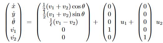
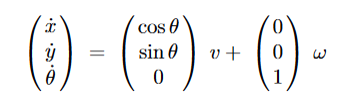
The reference point of the robot is the midpoint of the two wheels; its coordinates, with respect to a fixed frame, are denoted by (x,y) and θ is the direction of the driving wheels and ℓ is the distance between the driving wheels. By setting v=½*(v1+v2) and ω= 1/ℓ * (v1−v2) we get the kinematic model which is expressed as the following 3-dimensional system:

Car-like robots: The reference point with coordinates (x,y) is the midpoint of the rear wheels. We assume that the distance between both rear and front axles is unit length. We denote w as the speed of the front wheels of the car and ζ as the angle between the front wheels and the main direction θ of the car. Moreover a mechanical constraint imposes

ζ

≤ ζmax and consequently a minimum turning radius. The general dynamic model is given as:

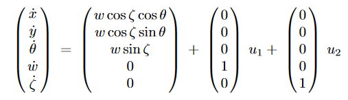
A first simplification consists in controlling w; it gives a 4-dimensional system. Let us assume that we do not care about the direction of the front wheels. We may still simplify the model. By setting v=wcosζ and ω=wsinζ we get a 3-dimensional system.

Sampling- vs Search-based Methods:

With constraints come some restrictions on the kinds of planners that will be effective. Grid-based graphs, for example, do not allow fluid motions to be planned but may work fine if a motion consisting of turn-in-place and drive straight maneuvers are acceptable. There are planners that incorporate simple fluid motions such as lattice planners, and Dubins and Reeds-Shepp state-space planners. The former of these can offer cheap planning for non-holonomic systems, so long as the number of extensions is kept low. The latter two present the space of options as arc and straight motions. These are typically for vehicles that use Ackerman steering. One alternative to all those above is a shooting RRT based on motion primitives. Where all of the others tend to work better at slower speeds, shooting RRTs can also work well at high speeds so long as the shooting is done using the vehicle dynamics. It may be possible to combine search-based with sampling-based planners in order to get optimality and feasibility benefits from both, respectively.

Detail Recommendations: Shooting RRT for High-speed Ackermann Vehicles

1. Consider distance metrics carefully:

Distance metrics are powerful tools to tune the planner by improving which node the planner chooses to expand. For example, it is better to choose a node that represents a state pointed in the direction of the sample but is slightly further by L2 distance than one pointed in the wrong direction. In this way, consider using a distance metric that makes L2 distance to the side of the vehicle more expensive. L2 distance behind the direction of motion could also be made expensive. Make sure to have a visualization of the distance metric for easier tuning.

2. Balance motion primitives:

Shots are typically taken over a certain period of time. What this means is that faster-accelerating shots that are pointed in the wrong direction can still make more progress than ones with more optimal directions.

3. Project speed limits from targets:

It can be time-consuming to convince a planner to slow down for a target depending on the implementation. If using backtracking as a method for slowing down, i.e. pruning back to a slower node, then this can take an exponential cost in number of iterations by the number of levels to backtrack. Instead, it is much faster to set local speed limits based on the distance to the target and the vehicle’s maximum deceleration.

4. Always slow down at the end of the path:

This is simply a safety concept and should help keep a run-away vehicle from happening.

5. One-pass planning:

Consider if the calculations used for shooting can be used for generating the final trajectory. This will save time in the form of not having to pass over the final path again. This is only really feasible if high frame rate trajectories are not strictly necessary.

References

[1] M. Likhachev. RI 16-782. Class Lecture, Topic:”Introduction; What is planning, Role of Planning in Robotics.” School of Computer Science, Carnegie Mellon University, Pittsburgh, PA, Aug. 26, 2019. https://www.cs.cmu.edu/~maxim/classes/robotplanning_grad/lectures/intro_16782_fall19.pdf

[2] M. Likhachev. RI 16-735. Class Lecture, Topic:”A* and Weighted A* Search.” School of Computer Science, Carnegie Mellon University, Pittsburgh, PA, Fall, 2010. https://www.cs.cmu.edu/~motionplanning/lecture/Asearch_v8.pdf

[3] C. A. Villegas, “Implementation, comparison, and advances in global planners using Ackerman motion primitives,” M. S. Thesis, Politencnico di Milano, Milan, IT, 2018. https://www.politesi.polimi.it/bitstream/10589/140048/3/2018_04_Arauz-Villegas.pdf

[4] S. Koenig and M. Lihachev, “D* Lite,” In Proc. of the AAAI Conference of Artificial Intelligence (AAAI), 2002, pp. 476-483. http://idm-lab.org/bib/abstracts/papers/aaai02b.pdf

[5] H. Choset.. RI 16-735. Class Lecture, Topic:”Robot Motion Planning: A* and D* Search.” School of Computer Science, Carnegie Mellon University, Pittsburgh, PA, Fall, 2010. https://www.cs.cmu.edu/~motionplanning/lecture/AppH-astar-dstar_howie.pdf

[6] J. Leavitt, B. Ayton, J. Noss, E. Harbitz, J. Barnwell, and S. Pinto. 16.412. Class Lecture, Topics: “Incremental Path Planning.” https://www.youtube.com/watch?v=_4u9W1xOuts

[7] I. Noreen, A. Khan, and Z. Habib, “A Comparison of RRT, RRT* and RRT*-Smart Path Planning Algorithms,” IJCSNS, vol. 16, no. 10, Oct., pp. 20-27, 2016. http://paper.ijcsns.org/07_book/201610/20161004.pdf

[8] J.P. Laumond, S. Sekhavat, and F. Lamiraux, “Guidelines in Nonholonomic Motion Planning for Mobile Robots,” in Robot Motion Planning and Control, J.P. Laumond, Eds. Berlin, Heidelberg: Springer Berlin Heidelberg, 1998, pp- 4-5.