Adaptive Monte Carlo Localization

What is a particle filter?

Particle filter are initialized by a very high number of particles spanning the entire state space. As you get additional measurements, you predict and update your measurements which makes your robot have a multi-modal posterior distribution. This is a big difference from a Kalman Filter which approximates your posterior distribution to be a Gaussian. Over multiple iterations, the particles converge to a unique value in state space.

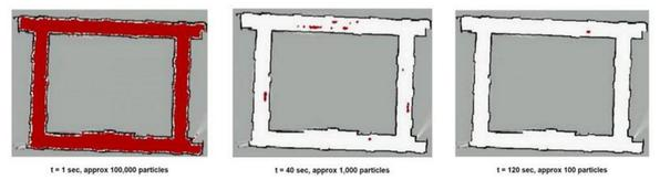
Figure 1: Particle Filter in Action over Progressive Time Steps

The steps followed in a Particle Filter are:

1. Re-sampling: Draw with replacement a random sample from the sample set according to the (discrete) distribution defined through the importance weights. This sample can be seen as an instance of the belief.

2. Sampling: Use previous belief and the control information to sample 􀀀from the distribution which describes the dynamics of the system. The current belief now represents the density given by the product of distribution and an instance of the previous belief. This density is the proposal distribution used in the next step.

3. Importance sampling: Weight the sample by the importance weight, the likelihood of the sample X given the measurement Z.

Each iteration of these three steps generates a sample drawn from the posterior belief. After n iterations, the importance weights of the samples are normalized so that they sum up to 1.

For further details on this topic, Sebastian Thrun’s paper on Particle Filter in Robotics is a good source for a mathematical understanding of particle filters, their applications and drawbacks.

What is an adaptive particle filter?

A key problem with particle filter is maintaining the random distribution of particles throughout the state space, which goes out of hand if the problem is high dimensional. Due to these reasons it is much better to use an adaptive particle filter which converges much faster and is computationally much more efficient than a basic particle filter.

The key idea is to bound the error introduced by the sample-based representation of the particle filter. To derive this bound, it is assumed that the true posterior is given by a discrete, piece-wise constant distribution such as a discrete density tree or a multidimensional histogram. For such a representation we can determine the number of samples so that the distance between the maximum likelihood estimate (MLE) based on the samples and the true posterior does not exceed a pre-specified threshold. As is finally derived, the number of particles needed is proportional to the inverse of this threshold.

Dieter Fox’s paper on Adaptive Particle Filters delves much deeper into the theory and mathematics behind these concepts. It also covers the implementation and performance aspects of this technique.

Use of Adaptive Particle Filter for Localization

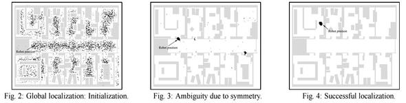
To use adaptive particle filter for localization, we start with a map of our environment and we can either set robot to some position, in which case we are manually localizing it or we could very well make the robot start from no initial estimate of its position. Now as the robot moves forward, we generate new samples that predict the robot’s position after the motion command. Sensor readings are incorporated by re-weighting these samples and normalizing the weights. Generally it is good to add few random uniformly distributed samples as it helps the robot recover itself in cases where it has lost track of its position. In those cases, without these random samples, the robot will keep on re-sampling from an incorrect distribution and will never recover. The reason why it takes the filter multiple sensor readings to converge is that within a map, we might have dis-ambiguities due to symmetry in the map, which is what gives us a multi-modal posterior belief.

Dieter Fox’s paper on Monte Carlo Localization for Mobile Robots gives further details on this topic and also compares this technique to many others such as Kalman Filter based Localization, Grid Based and Topological Markov Localization.

Configuring ROS AMCL package

At the conceptual level, the AMCL package maintains a probability distribution over the set of all possible robot poses, and updates this distribution using data from odometry and laser range-finders. Depth cameras can also be used to generate these 2D laser scans by using the package depthimage_to_laserscan which takes in depth stream and publishes laser scan on sensor_msgs/LaserScan. More details can be found on the ROS Wiki.

The package also requires a predefined map of the environment against which to compare observed sensor values. At the implementation level, the AMCL package represents the probability distribution using a particle filter. The filter is “adaptive” because it dynamically adjusts the number of particles in the filter: when the robot’s pose is highly uncertain, the number of particles is increased; when the robot’s pose is well determined, the number of particles is decreased. This enables the robot to make a trade-off between processing speed and localization accuracy.

Even though the AMCL package works fine out of the box, there are various parameters which one can tune based on their knowledge of the platform and sensors being used. Configuring these parameters can increase the performance and accuracy of the AMCL package and decrease the recovery rotations that the robot carries out while carrying out navigation.

There are three categories of ROS Parameters that can be used to configure the AMCL node: overall filter, laser model, and odometery model. The full list of these configuration parameters, along with further details about the package can be found on the webpage for AMCL. They can be edited in the amcl.launch file.

Here is a sample launch file. Generally you can leave many parameters at their default values.

<launch>

 <arg name="use_map_topic" default="false"/>
 <arg name="scan_topic" default="scan"/>

 <node pkg="amcl" type="amcl" name="amcl">
   <param name="use_map_topic" value="$(arg use_map_topic)"/>
   <!-- Publish scans from best pose at a max of 10 Hz -->
   <param name="odom_model_type" value="diff"/>
   <param name="odom_alpha5" value="0.1"/>
   <param name="gui_publish_rate" value="10.0"/>   <!-- 10.0 -->
   <param name="laser_max_beams" value="60"/>
   <param name="laser_max_range" value="12.0"/>
   <param name="min_particles" value="500"/>
   <param name="max_particles" value="2000"/>
   <param name="kld_err" value="0.05"/>
   <param name="kld_z" value="0.99"/>
   <param name="odom_alpha1" value="0.2"/>
   <param name="odom_alpha2" value="0.2"/>
   <!-- translation std dev, m -->
   <param name="odom_alpha3" value="0.2"/>
   <param name="odom_alpha4" value="0.2"/>
   <param name="laser_z_hit" value="0.5"/>
   <param name="laser_z_short" value="0.05"/>
   <param name="laser_z_max" value="0.05"/>
   <param name="laser_z_rand" value="0.5"/>
   <param name="laser_sigma_hit" value="0.2"/>
   <param name="laser_lambda_short" value="0.1"/>
   <param name="laser_model_type" value="likelihood_field"/>
   <!-- <param name="laser_model_type" value="beam"/> -->
   <param name="laser_likelihood_max_dist" value="2.0"/>
   <param name="update_min_d" value="0.25"/>
   <param name="update_min_a" value="0.2"/>
   <param name="odom_frame_id" value="odom"/>
   <param name="resample_interval" value="1"/>
   <!-- Increase tolerance because the computer can get quite busy -->
   <param name="transform_tolerance" value="1.0"/>
   <param name="recovery_alpha_slow" value="0.0"/>
   <param name="recovery_alpha_fast" value="0.0"/>
   <remap from="scan" to="$(arg scan_topic)"/>
 </node>
</launch>

Best way to tune these parameters is to record a ROS bag file, with odometry and laser scan data, and play it back while tuning AMCL and visualizing it on RViz. This helps in tracking the performance based on the changes being made on a fixed data-set.